In today's
session , we applied statistical knowledge gained in all the previous sessions
, in making power point presentation ,on our project topic "MONTH WISE
ARRIVALS OF FOREIGN TOURISTS IN INDIA" .We started with collection of data
from site www. Indiastat.com. We applied various suitable statistical measures
to interpret different facts . Statistical measures applied include mean , t-test
, correlation , regression.
MEAN
In probability and statistics, mean and expected value are used synonymous to refer to one measure of the central tendency either of a probability distribution or of the variable characterized by that distribution. In the case of a discrete probability distribution of a random variable X, the mean is equal to the sum over every possible value weighted by the probability of that value; that is, it is computed by taking the product of each possible value x of X and its probability P(x), and then adding all these products together, giving .
µ =Σ x P(x)
µ =Σ x P(x)
An analogous formula applies to the case of a continuous probability distribution. Not every probability distribution has a defined mean; see the Cauchy distribution for an example. Moreover, for some distributions the mean is infinite: for example, when the probability of the value is for n = 1, 2, 3, ....
For a data set, the terms arithmetic mean, mathematical expectation, and sometimes average are used synonymously to refer to a central value of a discrete set of numbers: specifically, the sum of the values divided by the number of values. T bar". If the data set were based on a series of observations obtained by sampling from a statistical population, the arithmetic mean is termed the sample mean to distinguish it from the population mean. .
For a finite population, the population mean of a property is equal to the arithmetic mean of the given property while considering every member of the population. For example, the population mean height is equal to the sum of the heights of every individual divided by the total number of individuals. The sample mean may differ from the population mean, especially for small samples. The law of large numbers dictates that the larger the size of the sample, the more likely it is that the sample mean will be close to the population mean.
DIAGRAM SHOWING COMPARISON OF MEAN , MEDIAN , MODE

t-test
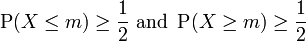
A t-test is any statistical hypothesis test in which the test statistic follows a Student's t distribution if the null hypothesis is supported. It can be used to determine if two sets of data are significantly different from each other, and is most commonly applied when the test statistic would follow a normal distribution if the value of a scaling term in the test statistic were known. When the scaling term is unknown and is replaced by an estimate based on the data, the test statistic (under certain conditions) follows a Student's t distribution.
Unpaired and paired two-sample t-test
Two-sample t-tests for a difference in mean involve independent samples, paired samples and overlapping samples. Paired t-tests are a form of blocking, and have greater power than unpaired tests when the paired units are similar with respect to "noise factors" that are independent of membership in the two groups being compared. In a different context, paired t-tests can be used to reduce the effects of confounding factors in an observational study.
(a) Independent samples
The independent samples t-test is used when two separate sets of independent and identically distributed samples are obtained, one from each of the two populations being compared. For example, suppose we are evaluating the effect of a medical treatment, and we enroll 100 subjects into our study, then randomize 50 subjects to the treatment group and 50 subjects to the control group. In this case, we have two independent samples and would use the unpaired form of the t-test. The randomization is not essential here—if we contacted 100 people by phone and obtained each person's age and gender, and then used a two-sample t-test to see whether the mean ages differ by gender, this would also be an independent samples t-test, even though the data are observational.
(b) Paired samples
Paired samples t-tests typically consist of a sample of matched pairs of similar units, or one group of units that has been tested twice (a "repeated measures" t-test).
A typical example of the repeated measures t-test would be where subjects are tested prior to a treatment, say for high blood pressure, and the same subjects are tested again after treatment with a blood-pressure lowering medication. By comparing the same patient's numbers before and after treatment, we are effectively using each patient as their own control. That way the correct rejection of the null hypothesis (here: of no difference made by the treatment) can become much more likely, with statistical power increasing simply because the random between-patient variation has now been eliminated. Note however that an increase of statistical power comes at a price: more tests are required, each subject having to be tested twice. Because half of the sample now depends on the other half, the paired version of Student's t-test has only 'n/2 - 1' degrees of freedom (with 'n' being the total number of observations). Pairs become individual test units, and the sample has to be doubled to achieve the same number of degrees of freedom.
A paired samples t-test based on a "matched-pairs sample" results from an unpaired sample that is subsequently used to form a paired sample, by using additional variables that were measured along with the variable of interest. The matching is carried out by identifying pairs of values consisting of one observation from each of the two samples, where the pair is similar in terms of other measured variables. This approach is sometimes used in observational studies to reduce or eliminate the effects of confounding factors.
Paired samples t-tests are often referred to as "dependent samples t-tests" (as are t-tests on overlapping samples).
(c) Overlapping samples
An overlapping samples t-test is used when there are paired samples with data missing in one or the other samples (e.g., due to selection of "Don't know" options in questionnaires or because respondents are randomly assigned to a subset question). These tests are widely used in commercial survey research (e.g., by polling companies) and are available in many standard crosstab software packages.
REGRESSION ANALYSIS
Regression analysis is a statistical process for estimating the relationships among variables. It includes many techniques for modeling and analyzing several variables, when the focus is on the relationship between a dependent variable and one or more independent variables. More specifically, regression analysis helps one understand how the typical value of the dependent variable changes when any one of the independent variables is varied, while the other independent variables are held fixed. Most commonly, regression analysis estimates the conditional expectation of the dependent variable given the independent variables – that is, the average value of the dependent variable when the independent variables are fixed. Less commonly, the focus is
In on a quantile, or other location parameter of the conditional distribution of the dependent variable given the independent variables. In all cases, the estimation target is a function of the independent variables called the regression function. In regression analysis, it is also of interest to characterize the variation of the dependent variable around the regression function, which can be described by a probability distribution.
Regression analysis is widely used for prediction and forecasting, where its use has substantial overlap with the field of machine learning. Regression analysis is also used to understand which among the independent variables are related to the dependent variable, and to explore the forms of these relationships. In restricted circumstances, regression analysis can be used to infer causal relationships between the independent and dependent variables.
DIAGRAM SHOWING REGRESSION ANALYSIS

X TABULATION:
There are several different types of correlation, and we’ll talk about them later, but in this lesson we’re going to spend most of the time on the most commonly used type of correlation: the Pearson Product Moment Correlation. This correlation, signified by the symbol r, ranges from –1.00 to +1.00. A correlation of 1.00, whether it’s positive or negative, is a perfect correlation. It means that as scores on one of the two variables increase or decrease, the scores on the other variable increase or decrease by the same magnitude—something you’ll probably never see in the real world. A correlation of 0 means there’s no relationship between the two variables, i.e., when scores on one of the variables go up, scores on the other variable may go up, down, or whatever. You’ll see a lot of those.
Thus, a correlation of .8 or .9 is regarded as a high correlation, i.e., there is a very close relationship between scores on one of the variables with the scores on the other. And correlations of .2 or .3 are regarded as low correlations, i.e., there is some relationship between the two variables, but it’s a weak one. Knowing people’s score on one variable wouldn’t allow you to predict their score on the other variable very well.
CORRELATION AND DEPENDENCE
In statistics, dependence refers to any statistical relationship between two random variables or two sets of data. Correlation refers to any of a broad class of statistical relationships involving dependence.
Familiar examples of dependent phenomena include the correlation between the physical statures of parents and their offspring, and the correlation between the demand for a product and its price. Correlations are useful because they can indicate a predictive relationship that can be exploited in practice. For example, an electrical utility may produce less power on a mild day based on the correlation between electricity demand and weather. In this example there is a causal relationship, because extreme weather causes people to use more electricity for heating or cooling; however, statistical dependence is not sufficient to demonstrate the presence of such a causal relationship (i.e., correlation does not imply causation).
Formally, dependence refers to any situation in which random variables do not satisfy a mathematical condition of probabilistic independence. In loose usage, correlation can refer to any departure of two or more random variables from independence, but technically it refers to any of several more specialized types of relationship between mean values. There are several correlation coefficients, often denoted ρ or r, measuring the degree of correlation. The commonest of these is the Pearson correlation coefficient, which is sensitive only to a linear relationship between two variables (which may exist even if one is a nonlinear function of the other). Other correlation coefficients have been developed to be more robust than the Pearson correlation – that is, more sensitive to nonlinear relationships. Mutual information can also be applied to measure dependence between two variables
DIAGRAM SHOWING FOUR SETS OF DATA SHOWING SAME CORRELATION

SUBMITTED BY : Pallavi Bizoara (2013186)
GROUP No : 7
Nidhi Sharma (2013169)
Nitesh Singh Patel(2013178)
Nitin Boratwar(2013179)
Palak Jain(2013185)


/Biostatistics/BIOSTATISTICS/Graphics/bs1.4.gif)


.jpg)


![\rho_{X,Y}=\mathrm{corr}(X,Y)={\mathrm{cov}(X,Y) \over \sigma_X \sigma_Y} ={E[(X-\mu_X)(Y-\mu_Y)] \over \sigma_X\sigma_Y},](http://upload.wikimedia.org/math/0/7/6/076d3820a46afe55ee680f3c85e34c76.png)